Invariant Manifolds
Invariant Manifolds are smooth manifolds that are invariant under a map or a flow. Any trajectory is obviously an invariant manifold, and the forward and backward trajectories through any set of points is invariant, but is not smooth.
One way to get a smooth manifold is using a transverse section [1]. A section is a smooth manifold which is transverse to the flow or map (the flow is tangent to the manifold, or for a map, the image of a point on the manifold is not on the manifold). For a smooth flow a $k-1$ dimensional transverse section the image of the section under the flow is a smooth $k$ dimensional manifold. For a smooth map the image of the section is another $k-1$ dimensional manifold.
For a map we might instead specify a smooth manifold between the section and its image under the map. The image of this manifold with boundary is not necessarily smooth on the section or its images. It's similar to delay differential equations, where initial conditions have to be specified on an interval. Here the interval is $k$-dimensional.
Suppose that the invariant manifold ${\cal M}$ is represented as an atlas of charts, each chart mapping a neighborhood of the origin in $\mathbb{R}^k$ onto ${\cal M}$. For a flow, invariance means that at each point a trajectory is some curve ${\bf u}({\bf s}(t))$, with ${\bf u}({\bf s})$ the chart mapping, and \begin{equation*} {\bf u}' = {\bf u}_{\bf s} {\bf s}' = {\bf F}({\bf u}({\bf s})). \end{equation*}
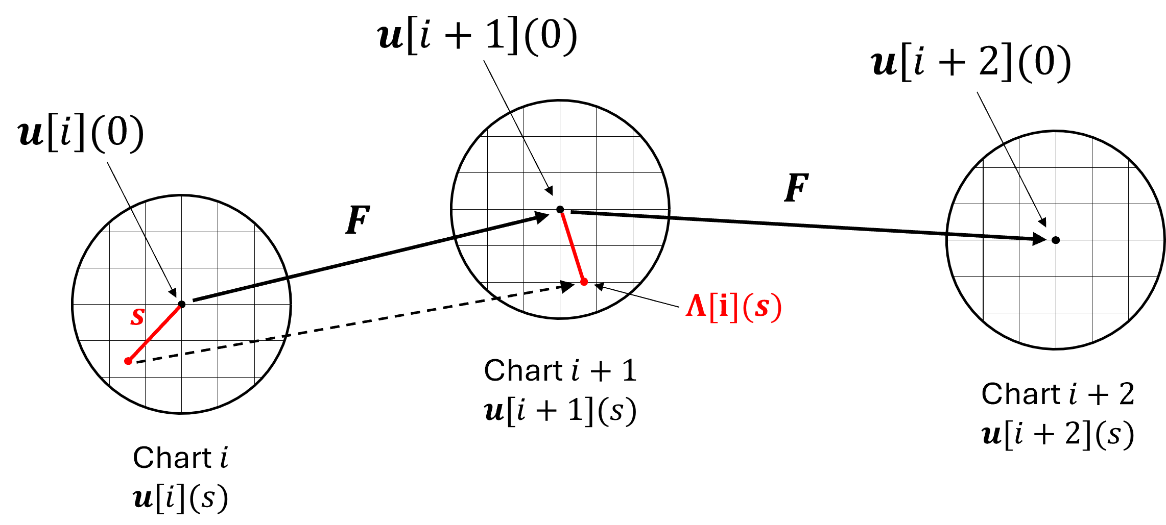
For a map things are a little more complicated, because a point can map to another chart. We might write \begin{equation*} {\bf F}({\bf u}({\bf s})) = {\bf u}(\Lambda({\bf s})) \end{equation*} with the understanding that $\Lambda$ may refer to a different chart, or something like \begin{equation*} {\bf F}({\bf u}[i]({\bf s}),{\bf s})) = {\bf u}[j({\bf s})](\Lambda[j]({\bf s})). \end{equation*} Typing and reading this gets old very quickly, so I'm going to shorten them where I can. Hopefully it will be clear in context.
In this document we first consider some cases where local analysis is possible, then computational approaches.
Local Analysis
There are some things that can be done analytically. Below we consider hyperbolic fixed points in maps and flows, for which a local analysis can be done, as well as trajectories in both maps and flows, where a different kind of local analysis is possible. In each case below Taylor series can be found for approximations local to fixed points and trajectories. As Jain and Haller [5] point out, these Taylor series approximations are Asymptotic Expansions. Truncated series are valid in some region about the origin, but that region may shrink to nothing as the number of terms in the series goes to infinity.
Taylor expansions of invariant manifolds in maps
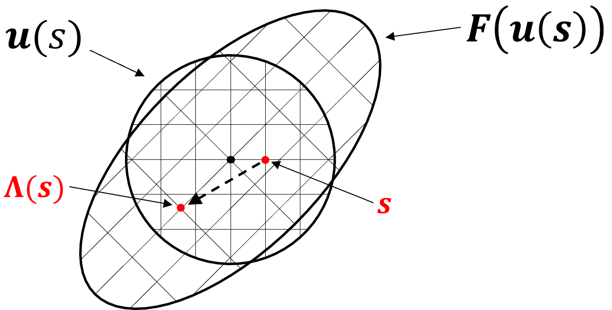
Suppose we have a map \begin{equation*} {\bf F}: {\bf u}\in\mathbb{R}^n\rightarrow {\bf F}({\bf u})\in\mathbb{R}^n. \end{equation*} For a set of local parameterizations of a manifold ${\bf u}[i]({\bf s})$ at iterates of the map to be invariant under the map we must have (for small $|{\bf s}|$) \begin{align} &{\bf u}[i+1](\Lambda[i+1]({\bf s})) = {\bf F}({\bf u}[i]({\bf s})) \nonumber \\ \tag{1}\label{1} \\ &{\left({\bf u}_{\bf s}[i+1](0)\right)}^T({\bf u}[i+1]({\bf s})-{\bf u}[i+1](0))={\bf s} \nonumber \end{align} I've used the tangent space at ${\bf s}=0$ at each point to parameterize the manifold. Note that ${\bf s}\in\mathbb{R}^k$ is a vector.
You can pretty easily compute a few terms in a Taylor series for ${\bf u}[i]({\bf s})$ and $\Lambda[i]({\bf s})$ [2], [3] , [4]. First let \begin{align} & {\bf u}[i]\equiv{\bf u}[i](0)\\ \\ & {\bf u}[i+1]\equiv{\bf u}(\Lambda[i](0))\\ \\ & \Lambda[i]\equiv\Lambda[i](0). \end{align} Differentiating the first equation in Equation $\eqref{1}$ with respect to ${\bf s}$, evaluating at the origin, and choosing $\Lambda[i](0)=0$, we get \begin{align} & {\bf u}[i+1] = {\bf F}\nonumber\\ \nonumber \\ &\begin{cases} {\bf u}_{\bf s}[i+1] \Lambda_{\bf s}[i+1] = {\bf F}_{\bf u} {\bf u}_{\bf s}[i] \\ \\ {\left( {\bf u}_{\bf s}[i+1]\right)}^T {\bf u}_{\bf s}[i+1] = I \\ \end{cases} \nonumber \\ \nonumber\\ &\begin{cases} {\bf u}_{\bf s}[i+1] \Lambda_{\bf ss}[i+1] + {\bf u}_{\bf ss}[i+1] \Lambda_{\bf s}[i+1] \Lambda_{\bf s}[i+1] = {\bf F}_{\bf u}{\bf u}_{\bf ss}[i] + {\bf F}_{\bf uu}{\bf u}_{\bf s}[i]{\bf u}_{\bf s}[i]\\ \\ {\left( {\bf u}_{\bf s}[i+1]\right)}^T {\bf u}_{\bf ss}[i+1] = 0 \end{cases} \tag{2}\label{2}\\ \nonumber \\ &\begin{cases} {\bf u}_{\bf s}[i+1] \Lambda_{\bf sss}[i+1] + 3 {\bf u}_{\bf ss}[i+1] \Lambda_{\bf s}[i+1] \Lambda_{\bf ss}[i+1] + {\bf u}_{\bf sss}[i+1] \Lambda_{\bf s}[i+1] \Lambda_{\bf s}[i+1] \Lambda_{\bf s}[i+1] = {\bf F}_{\bf uuu}{\bf u}_{\bf s}[i]{\bf u}_{\bf s}[i]{\bf u}_{\bf s}[i] + 3 {\bf F}_{\bf uu}{\bf u}_{\bf s}[i]{\bf u}_{\bf ss}[i] + {\bf F}_{\bf u}{\bf u}_{\bf sss}[i]. \\ \\ {\left( {\bf u}_{\bf s}[i+1]\right)}^T {\bf u}_{\bf sss}[i+1] = 0 \end{cases} \nonumber \end{align} The map ${\bf F}$ and its derivatives are evaluated at ${\bf u}[i](0)$. The expressions on both the left hand and right sides are the derivatives of a composition (``Faá di Bruno's Formula''). You can write out the general ${\rm n}^{\rm th}$ order equation if you really want. See Beyn and Kless [2]. Note that since ${\bf u}\in\mathbb{R}^n$ and ${\bf s}\in\mathbb{R}^k$, the derivatives are tensors, not scalars. The terms with coefficient three are sums of three different permutations of the indices: \begin{equation*} 3 {\bf F}_{\bf uu} {\bf u}_{\bf s} {\bf u}_{\bf ss} = \sum_p^{p\lt n}\sum_q^{q\lt n} \left( \frac{\partial F^i}{\partial u^p\partial u^q}\frac{\partial u^p}{\partial s^j}\frac{\partial^2 u^q}{\partial s^k \partial s^l} +\frac{\partial F^i}{\partial u^p\partial u^q}\frac{\partial u^p}{\partial s^k}\frac{\partial^2 u^q}{\partial s^j \partial s^l} +\frac{\partial F^i}{\partial u^p\partial u^q}\frac{\partial u^p}{\partial s^l}\frac{\partial^2 u^q}{\partial s^j \partial s^k} \right) \end{equation*} and \begin{equation*} 3 {\bf u}_{\bf ss}\Lambda_{\bf s} \Lambda_{\bf ss} = \sum_p^{p\lt n}\sum_q^{q\lt n} \left( \frac{\partial^2 u^i}{\partial s^p \partial s^q}\frac{\partial\Lambda^p}{\partial s^j}\frac{\partial^2 \Lambda^q}{\partial s^k \partial s^l} +\frac{\partial^2 u^i}{\partial s^p \partial s^q}\frac{\partial\Lambda^p}{\partial s^k}\frac{\partial^2 \Lambda^q}{\partial s^j \partial s^l} +\frac{\partial^2 u^i}{\partial s^p \partial s^q}\frac{\partial\Lambda^p}{\partial s^l}\frac{\partial^2 \Lambda^q}{\partial s^j \partial s^k} \right) \end{equation*}
We can split each of the equations $\eqref{2}$ by operating on the left with $\left( I-{\bf u}_{\bf s}[i+1] {\left( {\bf u}_{\bf s}[i+1]\right)}^T \right) $ and ${\left( {\bf u}_{\bf s}[i+1]\right)}^T$ in turn. Because the higher derivatives of ${\bf u}$ are required to be orthogonal to ${\bf u}_{\bf s}[i+1]$, operating with ${\left( {\bf u}_{\bf s}[i+1]\right)}^T$ eliminates all terms with the derivatives of $\Lambda$ except the highest, which will have a coefficient of one. Operating with $\left( I-{\bf u}_{\bf s}[i+1] {\left( {\bf u}_{\bf s}[i+1]\right)}^T\right) $ eliminates the term with the highest derivative of $\Lambda$. We get explicit expressions for the derivatives of $\Lambda$ \begin{align*} & \Lambda[i+1] = 0 \\ \\ & \Lambda_s[i+1] = {\left( {\bf u}_{\bf s}[i+1]\right)}^T {\bf F}_{\bf u}{\bf u}_{\bf s}[i] \\ \tag{3}\label{3}\\ & \Lambda_{ss}[i+1] = {\left( {\bf u}_{\bf s}[i+1]\right)}^T {\bf F}_{\bf u}{\bf u}_{\bf ss}[i] + {\left( {\bf u}_{\bf s}[i+1]\right)}^T {\bf F}_{\bf uu}{\bf u}_{\bf s}[i]{\bf u}_{\bf s}[i] \\ \\ & \Lambda_{\bf sss}[i+1] = {\left( {\bf u}_{\bf s}[i+1]\right)}^T {\bf F}_{\bf uuu}{\bf u}_{\bf s}[i]{\bf u}_{\bf s}[i]{\bf u}_{\bf s}[i] + 3 {\left( {\bf u}_{\bf s}[i+1]\right)}^T {\bf F}_{\bf uu}{\bf u}_{\bf s}[i]{\bf u}_{\bf ss}[i] + {\left( {\bf u}_{\bf s}[i+1]\right)}^T {\bf F}_{\bf u}{\bf u}_{\bf sss}[i] \end{align*} The equations for the derivatives of ${\bf u}$ depend on the situation.
Hyperbolic Fixed Points in maps
At a fixed point we have \begin{equation*} {\bf u}[i+1](0) = {\bf F}({\bf u}[i](0)). \qquad\qquad \Lambda[i](0)=0. \end{equation*} Since all the iterates are the same we can drop the index.
Applying $\left( I-{\bf u}_{\bf s} {\bf u}_{\bf s}^T\right)$ to equations [2] on the left, we have that \begin{align*} &\begin{cases} \left( I-{\bf u}_{\bf s} {\bf u}_{\bf s}^T\right){\bf F}_{\bf u}{\bf u}_{\bf s} = 0 \\ \\ {\bf u}_{\bf s}^T {\bf u}_{\bf s}=I \end{cases}\\ \\ &\begin{cases} \left( I-{\bf u}_{\bf s} {\bf u}_{\bf s}^T\right) {\bf F}_{\bf u}{\bf u}_{\bf ss} - {\bf u}_{\bf ss} \Lambda_{\bf s} \Lambda_{\bf s} = - \left( I-{\bf u}_{\bf s} {\bf u}_{\bf s}^T\right){\bf F}_{\bf uu}{\bf u}_{\bf s}{\bf u}_{\bf s} + {\bf u}_{\bf s} \Lambda_{\bf s} \\ \\ {\bf u}_{\bf s}^T {\bf u}_{\bf ss}=0 \end{cases}\\ \\ &\begin{cases} \left( I-{\bf u}_{\bf s} {\bf u}_{\bf s}^T\right) {\bf F}_{\bf u}{\bf u}_{\bf sss} - {\bf u}_{\bf sss} \Lambda_{\bf s} \Lambda_{\bf s} \Lambda_{\bf s} = - \left( I-{\bf u}_{\bf s} {\bf u}_{\bf s}^T\right) \left( {\bf F}_{\bf uuu}{\bf u}_{\bf s}{\bf u}_{\bf s}{\bf u}_{\bf s} + 3 {\bf F}_{\bf uu}{\bf u}_{\bf s}{\bf u}_{\bf ss} \right) + 3 {\bf u}_{\bf ss} \Lambda_{\bf s} \Lambda_{\bf ss} + {\bf u}_{\bf s} \Lambda_{\bf sss} \\ \\ {\bf u}_{\bf s}^T {\bf u}_{\bf sss}=0. \end{cases} \end{align*} These pairs are called Sylvester equations, of the form $AX+XB=C$. Beyn and Kless discuss ways of solving them. It looks like LAPACK v3 has routines for them (xTGSYL), though I haven't tried them. SciPy has a solve_sylvester routine. After finding ${\bf u}_{\bf s}$ we can use equations [3] to find $\Lambda_{\bf s}$ and then ${\bf u}_{\bf ss}$. The higher derivatives work the same way.
The first two equations require that ${\bf u}_{\bf s}$ be an o.n. basis for an invariant subspace (the image of the subspace spanned by ${\bf u}_{\bf s}$ has zero projection onto the orthogonal complement of the subspace).
A Neighborhood of a Trajectory in a map
If \begin{equation*} {\bf F}({\bf u}[i])\neq {\bf u}[i+1] \end{equation*} we still have $\Lambda[i](0)=0$.
Applying $\left( I-{\bf u}_{\bf s}[i+1] {\left( {\bf u}_{\bf s}[i+1]\right)}^T\right)$ to equations [2] on the left, collecting highest derivatives of ${\bf u}$ on the left, and adding the parameterization, we have that \begin{align*} &\begin{cases} \left( I-{\bf u}_{\bf s}[i+1] {\left( {\bf u}_{\bf s}[i+1]\right)}^T\right) {\bf F}_{\bf u}{\bf u}_{\bf s}[i] = 0 \\ \\ {\left( {\bf u}_{\bf s}[i+1]\right)}^T {\bf u}_{\bf s}[i+1]=I \end{cases} \\ \\ &\begin{cases} {\bf u}_{\bf ss}[i+1] \Lambda_{\bf s}[i+1] \Lambda_{\bf s}[i+1] \\ \\ \qquad\qquad\qquad\qquad = \left( I-{\bf u}_{\bf s}[i+1] {\left( {\bf u}_{\bf s}[i+1]\right)}^T\right) \left( {\bf F}_{\bf u}{\bf u}_{\bf ss}[i] + {\bf F}_{\bf uu}{\bf u}_{\bf s}[i]{\bf u}_{\bf s}[i] \right) - {\bf u}_{\bf s}[i+1] \Lambda_{\bf s}[i+1] \\ \\ {\left({\bf u}_{\bf s}[i+1] \right)}^T {\bf u}_{\bf ss}[i+1]=0\\ \end{cases} \\ \\ &\begin{cases} {\bf u}_{\bf sss}[i+1] \Lambda_{\bf s}[i+1] \Lambda_{\bf s}[i+1] \Lambda_{\bf s}[i+1]\\ \\ \qquad\qquad\qquad\qquad = \left( I-{\bf u}_{\bf s}[i+1] {\left( {\bf u}_{\bf s}[i+1]\right)}^T\right) \left( {\bf F}_{\bf u}{\bf u}_{\bf sss}[i] + 3 {\bf F}_{\bf uu}{\bf u}_{\bf s}[i]{\bf u}_{\bf ss}[i] + {\bf F}_{\bf uuu}{\bf u}_{\bf s}[i]{\bf u}_{\bf s}[i]{\bf u}_{\bf s}[i] \right) \\ \\ \qquad\qquad\qquad\qquad\qquad\qquad - 3 {\bf u}_{\bf ss}[i+1] \Lambda_{\bf s}[i+1] \Lambda_{\bf ss}[i+1] \\ \\ {\left( {\bf u}_{\bf s}[i+1]\right)}^T {\bf u}_{\bf sss}[i+1]=0. \end{cases} \end{align*} The first pair require that ${\bf u}_{\bf s}[i+1]$ be an o.n. basis for the subspace spanned by the columns of ${\bf F}_{\bf u}({\bf u}[i]){\bf u}_{\bf s}[i]$, (the image of the subspace spanned by ${\bf u}_{\bf s}[i]$ has zero projection onto the orthogonal complement of the span of ${\bf u}_{\bf s}[i+1]$). ${\bf u}_{\bf s}[i+1]$ can be found by mapping ${\bf u}_{\bf s}[i]$ and using Gram-Schmidt. With it $\Lambda_{\bf s}[i+1]$ can be found using the first equation in $\eqref{3}$, then the second pair of equations above can be solved for ${\bf u}_{\bf ss}[i+1]$ and so on. $\Lambda_{\bf s}[i+1]$ is square ($k\times k$), and represents how the map transforms parameters. So it is presumably invertible, making finding ${\bf u}_{\bf ss}[i+1]$ and the higher derivatives straight forward.
Note that unlike near the fixed point, the initial subspace ${\bf u}_{\bf s}[0]$ and higher derivatives have no restrictions. The map iterates any small patch (submanifold of phase space) forward. If the iterates lie on a cycle, say ${\bf u}[N-1]={\bf u}[0]$, then ${\bf u}_{\bf s}[N-1]$ and ${\bf u}_{\bf s}[0]$ must span the same subspace, which determines that subspace.
Taylor expansions of invariant manifolds in flows
Suppose we have a flow \begin{equation*} {\bf u}'={\bf F}({\bf u}), \qquad\qquad {\bf F}:\mathbb{R}^n\rightarrow\mathbb{R}^n, \end{equation*} which has a manifold which is invariant under the flow with a local parameterization ${\bf u}({\bf s})$ about a point ${\bf u}(0)$. If the manifold is invariant, a trajectory starting at ${\bf u}(0)$ is some path ${\bf u}({\bf s}(t))$ on the manifold with \begin{equation*} {\bf u}'={\bf u}_{\bf s}{\bf s}' = {\bf F}({\bf u}({\bf s})). \end{equation*} If we call the dynamics on the manifold ${\bf a}({\bf s})$ (in the local parameterization), we have \begin{equation*} {\bf s}'={\bf a}({\bf s}). \end{equation*} With a local parameterization this gives us the equations \begin{align*} & {\bf u}_{\bf s}{\bf a} = {\bf F}\\ \\ & {\left( {\bf u}_{\bf s}(0)\right)}^T\left( {\bf u}({\bf s}) - {\bf u}(0)\right) = {\bf s}. \end{align*} The flow ${\bf s}'={\bf a}({\bf s})$ is the analog of the map ${\bf s}\rightarrow\Lambda({\bf s})$ for the map.
We can find equations for the derivatives of ${\bf u}$ and ${\bf a}$ with respect to ${\bf s}$ at the origin by differentiating \begin{align} &\begin{cases} {\bf u}_{\bf s}{\bf a} = {\bf F} \\ \\ {\bf u}_{\bf s}^T {\bf u}_{\bf s} = I \end{cases} \nonumber \\ \\ &\begin{cases} {\bf u}_{\bf s}{\bf a}_{\bf s} + {\bf u}_{\bf ss}{\bf a} = {\bf F}_{\bf u} {\bf u}_{\bf s}\\ \\ {\bf u}_{\bf s}^T {\bf u}_{\bf ss} = 0 \end{cases} \tag{4}\label{4} \\ \\ &\begin{cases} {\bf u}_{\bf s}{\bf a}_{\bf ss} + 2 {\bf u}_{\bf ss}{\bf a}_{\bf s} + {\bf u}_{\bf sss}{\bf a} = {\bf F}_{\bf uu} {\bf u}_{\bf s} {\bf u}_{\bf s} + {\bf F}_{\bf u} {\bf u}_{\bf ss} \\ \\ {\bf u}_{\bf s}^T {\bf u}_{\bf sss} = 0 \end{cases} \nonumber \\ \\ &\begin{cases} {\bf u}_{\bf s}{\bf a}_{\bf sss} + 3 {\bf u}_{\bf ss}{\bf a}_{\bf ss} + 3 {\bf u}_{\bf sss}{\bf a}_{\bf s} + {\bf u}_{\bf ssss}{\bf a} = {\bf F}_{\bf uuu} {\bf u}_{\bf s} {\bf u}_{\bf s} {\bf u}_{\bf s} +3 {\bf F}_{\bf uu} {\bf u}_{\bf ss} {\bf u}_{\bf s} + {\bf F}_{\bf u} {\bf u}_{\bf sss} \\ \\ {\bf u}_{\bf s}^T {\bf u}_{\bf ssss} = 0. \end{cases} \end{align} These are very similar to Equation $\eqref{2}$. However, the expression on the left is the derivative of a product instead of a composition (the ``General Leibniz Rule''). Note that \begin{equation*} 2 {\bf u}_{\bf ss}{\bf a}_{\bf s}= \frac{\partial^2 u^i}{\partial s^p\partial s^k} \frac{\partial a^p}{\partial s^j} + \frac{\partial^2 u^i}{\partial s^p\partial s^j} \frac{\partial a^p}{\partial s^k} \end{equation*} and \begin{align*} & 3 {\bf u}_{\bf ss}{\bf a}_{\bf ss}= \frac{\partial^2 u^i}{\partial s^p\partial s^j} \frac{\partial^2 a^p}{\partial s^k\partial s^l} +\frac{\partial^2 u^i}{\partial s^p\partial s^k} \frac{\partial^2 a^p}{\partial s^j\partial s^l} +\frac{\partial^2 u^i}{\partial s^p\partial s^l} \frac{\partial^2 a^p}{\partial s^j\partial s^k}\\ \\ & 3 {\bf u}_{\bf sss}{\bf a}_{\bf s}= \frac{\partial^3 u^i}{\partial s^p\partial s^j\partial s^k} \frac{\partial a^p}{\partial s^l} +\frac{\partial^3 u^i}{\partial s^p\partial s^j\partial s^l} \frac{\partial a^p}{\partial s^k} +\frac{\partial^3 u^i}{\partial s^p\partial s^k\partial s^l} \frac{\partial a^p}{\partial s^j}. \end{align*}
The orthogonality of higher derivatives of ${\bf u}$ means that operating on the left with ${\bf u}_{\bf s}^T$ eliminates all but the highest derivatives of ${\bf a}$, which will have a coeficient of one. As with $\Lambda$ for the map this produces explicit equations for ${\bf a}$ and derivatives \begin{align} & {\bf a} = {\bf u}_{\bf s}^T{\bf F} \nonumber \\ \nonumber \\ & {\bf a}_{\bf s} = {\bf u}_{\bf s}^T {\bf F}_{\bf u} {\bf u}_{\bf s} \nonumber \\ \tag{5}\label{5}\\ & {\bf a}_{\bf ss} = {\bf u}_{\bf s}^T {\bf F}_{\bf uu} {\bf u}_{\bf s} {\bf u}_{\bf s} + {\bf u}_{\bf s}^T {\bf F}_{\bf u} {\bf u}_{\bf ss} \nonumber \\ \\ & {\bf a}_{\bf sss} = {\bf u}_{\bf s}^T {\bf F}_{\bf uuu} {\bf u}_{\bf s} {\bf u}_{\bf s} {\bf u}_{\bf s} +3 {\bf u}_{\bf s}^T {\bf F}_{\bf uu} {\bf u}_{\bf s} {\bf u}_{\bf ss} + {\bf u}_{\bf s}^T {\bf F}_{\bf u} {\bf u}_{\bf sss}. \nonumber \end{align} The equations for the derivatives of ${\bf u}$ depend on the situation.
Hyperbolic Fixed Points in flows
At a hyperbolic fixed point ${\bf F}({\bf u}(0))=0$ and the first equation in Equation $\eqref{5}$ becomes \begin{equation*} {\bf a} = {\bf u}_{\bf s}^T{\bf F} \longrightarrow {\bf a} = 0. \end{equation*} Applying $(I-{\bf u}_{\bf s}{\bf u}_{\bf s}^T)$ to the equations for the derivatives of ${\bf u}$ and ${\bf a}$ with respect to ${\bf s}$ $\eqref{4}$ eliminates the highest derivatives of ${\bf a}$. Rearranging to collect the highest derivatives of ${\bf u}$ on the left, we have \begin{align*} &\begin{cases} (I-{\bf u}_{\bf s}{\bf u}_{\bf s}^T) {\bf F}_{\bf u} {\bf u}_{\bf s} = 0 \\ \\ {\bf u}_{\bf s}^T {\bf u}_{\bf s}= I \end{cases} \\ \\ &\begin{cases} (I-{\bf u}_{\bf s}{\bf u}_{\bf s}^T) {\bf F}_{\bf u} {\bf u}_{\bf ss} - 2 {\bf u}_{\bf ss}{\bf a}_{\bf s} = - (I-{\bf u}_{\bf s}{\bf u}_{\bf s}) {\bf F}_{\bf uu} {\bf u}_{\bf s} {\bf u}_{\bf s} \\ \\ {\bf u}_{\bf s}^T {\bf u}_{\bf ss}= 0 \end{cases} \\ \\ &\begin{cases} (I-{\bf u}_{\bf s}{\bf u}_{\bf s}^T) {\bf F}_{\bf u} {\bf u}_{\bf sss} - 3 {\bf u}_{\bf sss}{\bf a}_{\bf s} = \\ \\ \qquad\qquad\qquad - (I-{\bf u}_{\bf s}{\bf u}_{\bf s}^T) \left( {\bf F}_{\bf uuu} {\bf u}_{\bf s} {\bf u}_{\bf s} {\bf u}_{\bf s} + 3 {\bf F}_{\bf uu} {\bf u}_{\bf ss} {\bf u}_{\bf s}\right) + 3 {\bf u}_{\bf ss}{\bf a}_{\bf ss}\\ \\ {\bf u}_{\bf s}^T {\bf u}_{\bf sss}= 0. \end{cases} \end{align*} The first pair say that ${\bf u}_{\bf s}$ is an orthonormal basis for an invariant subspace of the Jacobian ${\bf F}_{\bf u}$ (the image of the subspace spanned by ${\bf u}_{\bf s}$ has no projection orthogonal to ${\bf u}_{\bf s}$).
A Neighborhood of a Trajectory in a Flow
If $|{\bf F}({\bf u}(0))|>0$ we have a point on some unknown manifold that is invariant under the flow. Applying $(I-{\bf u}_{\bf s}{\bf u}_{\bf s}^T)$ to equations $\eqref{4}$ eliminates the highest derivatives of ${\bf a}$. Rearranging to collect the highest derivatives of ${\bf u}$, we have \begin{align*} & (I-{\bf u}_{\bf s}{\bf u}_{\bf s}^T) {\bf F} = 0 \\ \\ & {\bf u}_{\bf ss}{\bf a} = (I-{\bf u}_{\bf s}{\bf u}_{\bf s}^T) {\bf F}_{\bf u} {\bf u}_{\bf s} \\ \\ & {\bf u}_{\bf sss}{\bf a} = (I-{\bf u}_{\bf s}{\bf u}_{\bf s}^T) \left( {\bf F}_{\bf uu} {\bf u}_{\bf s} {\bf u}_{\bf s} + {\bf F}_{\bf u} {\bf u}_{\bf ss} \right) - 2 {\bf u}_{\bf ss}{\bf a}_{\bf s} \\ \\ & {\bf u}_{\bf ssss}{\bf a} = (I-{\bf u}_{\bf s}{\bf u}_{\bf s}^T) \left( {\bf F}_{\bf uuu} {\bf u}_{\bf s} {\bf u}_{\bf s} {\bf u}_{\bf s} +3 {\bf F}_{\bf uu} {\bf u}_{\bf ss} {\bf u}_{\bf s} + {\bf F}_{\bf u} {\bf u}_{\bf sss}\right) - 3 {\bf u}_{\bf ss}{\bf a}_{\bf ss} - 3 {\bf u}_{\bf ss}{\bf a}_{\bf s}. \end{align*} The first equation states that the tangent space must contain the flow. If we recognize that the left hand sides are the time derivatives of the derivatives of ${\bf u}$ ($d/dt = d/d{\bf s}~{\bf s}'$) the remaining equations are ODE's for the derivatives of ${\bf u}$ \begin{align*} & {({\bf u}_{\bf s})}' = (I-{\bf u}_{\bf s}{\bf u}_{\bf s}^T) {\bf F}_{\bf u} {\bf u}_{\bf s} \\ \\ & {({\bf u}_{\bf ss})}' = (I-{\bf u}_{\bf s}{\bf u}_{\bf s}^T) \left( {\bf F}_{\bf uu} {\bf u}_{\bf s} {\bf u}_{\bf s} + {\bf F}_{\bf u} {\bf u}_{\bf ss} \right) - 2 {\bf u}_{\bf ss}{\bf a}_{\bf s} \\ \\ & {({\bf u}_{\bf sss})}' = (I-{\bf u}_{\bf s}{\bf u}_{\bf s}^T) \left( {\bf F}_{\bf uuu} {\bf u}_{\bf s} {\bf u}_{\bf s} {\bf u}_{\bf s} +3 {\bf F}_{\bf uu} {\bf u}_{\bf ss} {\bf u}_{\bf s} + {\bf F}_{\bf u} {\bf u}_{\bf sss}\right) - 3 {\bf u}_{\bf ss}{\bf a}_{\bf ss} - 3 {\bf u}_{\bf ss}{\bf a}_{\bf s}. \end{align*} These are the equations for an augmented (fattened) trajectory which were derived in [6].
Note also that the right hand sides are orthogonal to ${\bf u}_{\bf s}$. That means that if ${\bf u}_{\bf s}$ is orthonormal at ${\bf s}=0$, and the second and higher derivatives of ${\bf u}$ are orthogonal to ${\bf u}_{\bf s}$ at ${\bf s}=0$ (the initial parameterization is locally Euclidean), it remains so \begin{equation*} {({\bf u}_{\bf s}^T{\bf u}_{\bf s})}'=2{\bf u}_{\bf s}^T {\bf u}_{\bf s}' = 0. \end{equation*}
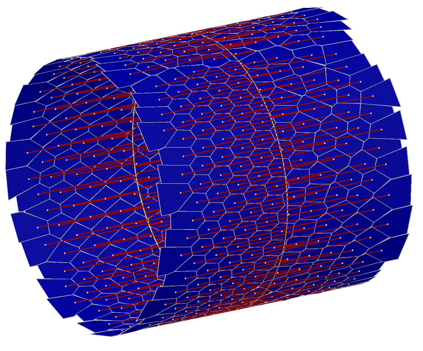
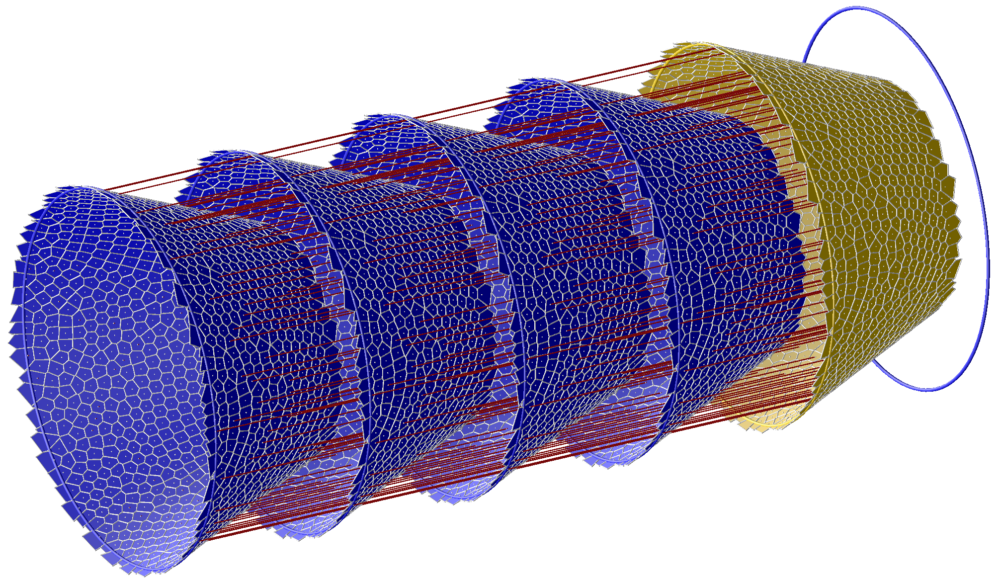
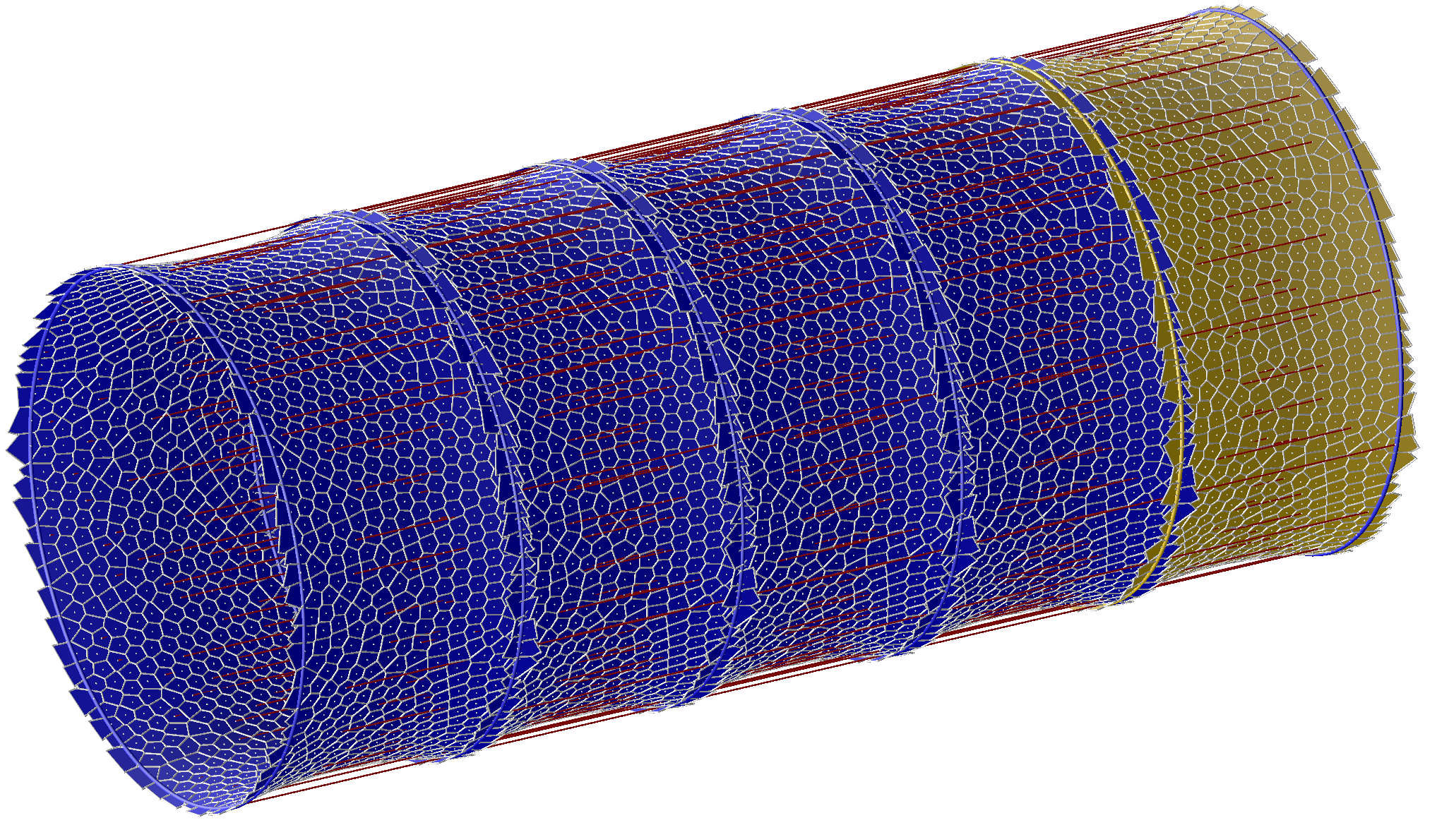
Computing invariant manifolds of fixed points
We can write a point on the invariant manifold of a fixed point ${\bf u}^*$ with an invariant subspace as the solution of a two point boundary value problem. For a flow \begin{align*} & {\bf u}' = T {\bf F}({\bf u})\\ \\ & \left(I-{\bf u}_{\bf s}^* {({\bf u}_{\bf s}^*)}^T\right)\left( {\bf u}(0)-{\bf u}^*\right)=0\\ \\ &{\left({\bf u}(0)-{\bf u}^*\right)}^T \left({\bf u}(0)-{\bf u}^*\right)=R^2, \end{align*} and for a map \begin{align*} & {\bf u}[i+1] = {\bf F}({\bf u}[i]) \\ \\ & \left(I-{\bf u}_{\bf s}^* {({\bf u}_{\bf s}^*)}^T\right)\left( {\bf u}[0]-{\bf u}^*\right)=0\\ \\ &{\left({\bf u}[0]-{\bf u}^*\right)}^T \left({\bf u}[0]-{\bf u}^*\right)\leq R^2,\\ \\ &{\left({\bf u}[1]-{\bf u}^*\right)}^T \left({\bf u}[1]-{\bf u}^*\right)>R^2. \end{align*} This uses a linear approximation for the unstable manifold, higher order could be used. That would be somthing like \begin{align*} &{\bf s}(0) = {({\bf u}_{\bf s}^*)}^T \left( {\bf u}(0)-{\bf u}^*\right) \\ \\ & \left(I-{\bf u}_{\bf s}^* {({\bf u}_{\bf s}^*)}^T\right)\left( {\bf u}(0)-{\bf u}^*\right) = \frac{1}{2} {\bf u}_{\bf ss}^* {\bf s}(0) {\bf s}(0). \end{align*}
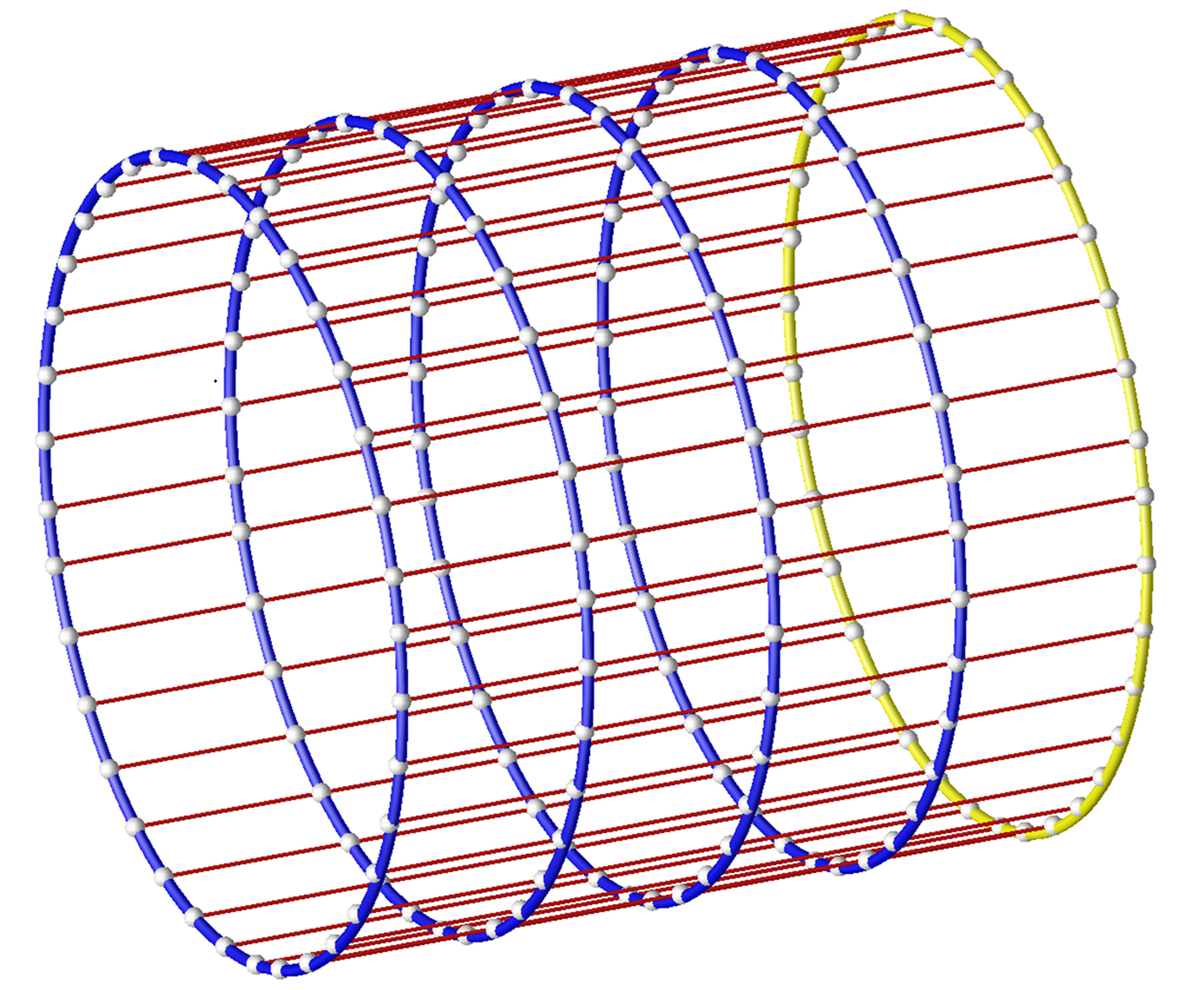
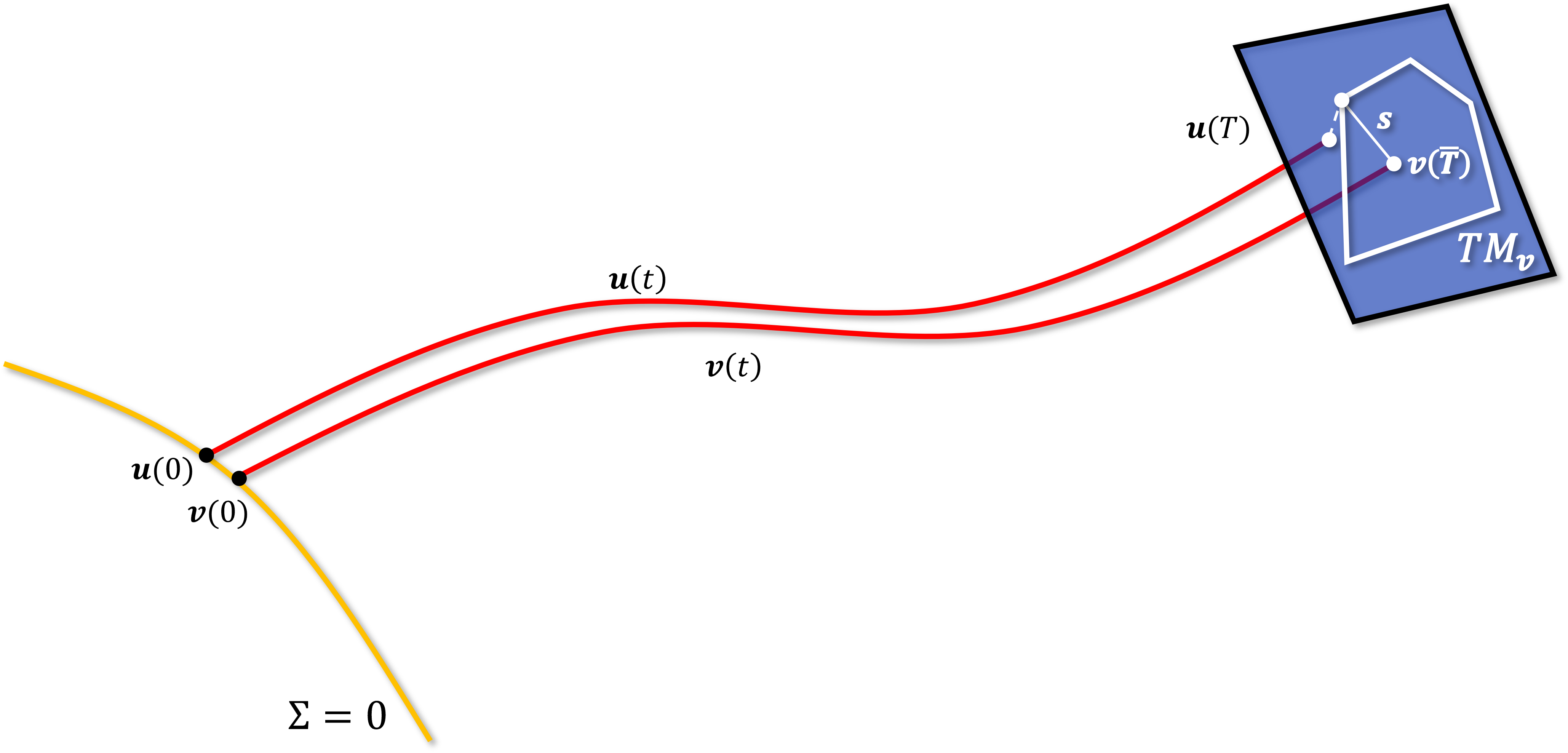
To find a point on the invariant manifold we follow the approach in [7]. We assume that we have a point ${\bf v}$, the tangent space $\Phi$, and the associated trajectory ${\bf v}(t)$ connecting ${\bf v}$ back to $\Sigma=0$. For a flow this will be a trajectory ${\bf v}(t)$, $t\in[0,\bar T]$ and for a map a trajectory ${\bf v}[i]$ for $i\in[0,N]$. A point near ${\bf v}$ on the invariant manifold, at parameter value ${\bf s}$, will lie on a trajectory ${\bf u}(t)$ that satisfies the end condition \begin{equation*} \Phi^T\left( {\bf u}(T)-{\bf v}(\bar T)\right) = {\bf s}, \end{equation*} or, for the map, \begin{equation*} \Phi^T\left( {\bf u}[N]-{\bf v}[N]\right) = {\bf s}. \end{equation*}
The ``project'' operation consists of solving for the new trajectory ${\bf u}$. The tangent space of the invariant manifold can be found by integrating the or mapping the tangent space on $\Sigma=0$, as can the curvature. We would recommend instead storing an augmented trajectory for tangent and curvature instead of just ${\bf v}(t)$, and solving for an augmented trajectory in the ``project'' operation. The tangent space and curvature can then be found trivially.
[1] William Basener, "Every nonsingular C1 flow on a closed manifold of dimension greater than two has a global transverse disk", Topology and its Applications 135(1-3), pp. 131-148, 2004.
[2] W.-J. Beyn and W. Kless, "Numerical Taylor expansions of invariant manifolds in large dynamical systems", Numerische Mathematik, 80 (1998), pp. 1–38.
[3] X. Cabr´e, E. Fontich, and R. De La Llave, "The parameterization method for invariant manifolds III: overview and applications", Journal of Differential Equations, 218 (2005), pp. 444–515.
[4] Timo Eirola, Jan von Pfaler, "Numerical Taylor expansions for invariant manifolds". Numer. Math. 99, 25–46 (2004)
[5] Shobit Jain, George Haller, “How to Compute Invariant Manifolds and Their Reduced Dynamics in High-Dimensional Finite Element Models.”. Nonlinear Dynamics 107, no. 2 (2022).
[6] Michael E. Henderson, "Computing Invariant Manifolds by Integrating Fat Trajectories", SIAM J. Appl. Dyn. Sys., 4(4), pp. 832-882, 2005.
[7] Michael E. Henderson, "Multiple Parameter Continuation: Computing Implicitly Defined k-manifolds", IJBC v12(3), pp 451-76.
Michael E. Henderson michael.e.henderson.10590 at gmail.com